Many Reinforcement Learning (RL) algorithms assume that a reward function is known (or can be obtained by interacting with the environment). However, it is hard to define such a reward function that leads to desired behaviors in many cases. It could be due to sparse reward, high dimensionality, etc. There is a gap between human understanding of reward and the way that RL algorithm finds policy based on the reward. Therefore, it will be beneficial to be able to determine reward function from human demonstration. It is similar to a translator that converts human intent to a robot’s reward function. Moreover, by extracting the reward function from human demonstrations, we will also be able to infer the human preference. For example, a human demonstrator might like moving very close to a wall when approaching the goal. An agent can learn from demonstration to have a higher reward close to the wall but still maintain the appropriate weight ratio with respect to the goal reward, which ends up leading the agent to the goal along the wall. Even when the environment has changed (wall position has changed), the agent can still move with the same preference (closed to the wall), which is the ability to generalize to a novel configuration of the environment. With such a reward function, we can predict human behavior based on preference for similar environments. Another example would be in autonomous driving where the vehicle can learn human driving preference and mimic similar behavior to generate a preferred and comfortable driving trajectory.
This project uses Maximum Entropy Deep Inverse Reinforcement Learning (IRL) with Soft Actor-Critic (SAC) to determine a reward function representing user preference during a continuous path planning scenario. The scenario came up when I walked by a trash can one time, and I was disgusted by the smell. The next time I walked by the same place, I intentionally avoided the trash can (that’s my preference). Figure 1 shows an example. There is a room that has perfumes, natural flowers, and a trash bag. A person needs to navigate through perfumes, flowers, or trash bags in order to reach his/her goal. These objects have different smells which correspond to different preferences when the person chooses a path: Some people like natural smell from flowers, some people like artificial smell from perfumes, and some people might be ok with trash bag smell as long as they can get to the goal. However, we don’t have this information as a prior; we need to infer the preference based on the person’s behavior.
![](/images/irl/example.png) |
---|
*Figure 1. An Example Scenario* |
The high-level plan is to take a demonstrated path. We then use IRL to extract a reward function from the demonstration for this 2D continuous space. After that, we can use the reward function with standard RL to predict the human preferred path next time he/she enters the room, even when the positions of the objects have changed.
The IRL algorithm used in this project is a modified version of the paper Maximum Entropy Deep Inverse Reinforcement Learning by Wulfmeier et al. in 2016[1]. I will discuss a short version of the algorithm formulation here. For more detail information, please refer to the paper. The following notations are also taken from the paper[1]
In standard RL, we assume a Markov Decision Process (MDP) that is defined by state $S$, action $A$, transition model $T$, and the reward $r$. The policy $\pi$ that maximizes the expected reward is the optimal policy $\pi^{*}$. In IRL, we are interested in the inverse problem: The policy $\pi$ is given which will be used to determine the reward $r$.
How do we express the reward function? In many of the previous IRL algorithms, the reward function is represented by a linear combination of the features.
$$r = \theta^{T}f$$
where $\theta$ is the weight vector and $f$ is the feature vector. The form of Linear combination will limit the ways of representing reward functions since there could be rewards that cannot be approximated by linear formulation. In order to be more generalized to nonlinear reward functions, we can use neural network as a nonlinear function approximators. This is where the term “Deep” comes up in this algorithm compared to its predecessor Maximum Entropy IRL by Ziebart et al. in 2008[2]. The reward function now becomes:
$$r=g(f, \theta_{1}, \theta_{2}, …)$$
where $\theta_{n}$ are just the network parameters in the neural network.
To solve the IRL problem, we will maximize the joint posterior distribution of the demonstration $D$ and the network parameters given the reward function:
$$ L(\theta)=\log P(D, \theta \mid r) = \log P(D \mid r) + \log P(\theta) = L_{D} + L_{\theta}$$
Since it is differentiable with respect to $\theta$, we can take the gradient with respect to $\theta$ and use gradient descent.
$$ \frac{\partial L}{\partial \theta}=\frac{\partial L_{D}}{\partial \theta}+\frac{\partial L_{\theta}}{\partial \theta} $$
The first term can be further decomposed into:
$$ \frac{\partial L_{D}}{\partial \theta}=\frac{\partial L_{D}}{\partial r} \cdot \frac{\partial r}{\partial \theta} $$
Based on the the original Maximum Entropy IRL [2]:
$$ \frac{\partial L_{D}}{\partial r} = \left(\mu_{D}-\mathbb{E}[\mu]\right) $$
which is the difference between the expert demonstration features trajectories and the expected current policy features trajectories. The difference here can be used as the error that starts the back propagation.
The implementation is based on the algorithm given by the original paper as shown in Figure 2 with modifications.
![](/images/irl/code.png) |
---|
*Figure 2. Full Algorithm* |
The modifications happen at line 4 and line 5 in Figure 2. Line 4 is used for determining the current optimal policy given the current reward function. Line 5 is for generating expected state features based on the current optimal policy. However, the original paper uses value iteration to find the optimal policy, which is difficult in a continuous environment. To adapt to continuous environment and possibly expand to other future robotics applications, I decided to use Soft Actor-Critic (SAC) as the method to find the optimal policy with the current reward function. The complete pipeline is shown in Figure 3
![](/images/irl/pipeline.png) |
---|
*Figure 3. Full Pipeline for Training* |
The pipeline can be described as the following steps:
The network we will be using is a two-layer network with 64 nodes as the hidden states for each layer.
As briefly introduced in the previous section, the scenario will be described in more details here. Figure 4 shows the example scenario again. It is a rectagular 2D continuous space. A human starting from the right side (the blue dot) can take continuous actions to reach the goal (the green dot) on the left side. The human will need to go through two layers of objects including perfumes, flowers, and trash bag. Each of these objects will have different smells which only diffuse to a circular area around the object, and there is no intersection between the smells. The color shows the area each smell covers. The first layer is covered by sakura flowers, perfume 1, and a trash bag (from the top to the bottom). The second layer does not have the trash bag, it is only covered by roses and perfume 2 (from the top to the bottom). A person will navigate to the goal based on his/her preference of smells.
![](/images/irl/input.png) |
---|
*Figure 4. An Example Scenario* |
To perform the smell room experiment, I first created a game interface for collecting user demonstration using Pygame. A user can use a gaming controller joystick as the input for creating demonstration. Figure 5 shows an example of a user moving freely in the room with a joystick. Once the user thinks the demonstration is complete, the user can close the pygame window, which the trajectory will be recorded.
![](/images/irl/pygame.gif) |
---|
*Figure 5. The Pygame Interface* |
One example of the demonstration path is shown in Figure 6. We will proceed with this demonstration for the rest of the experiment. From this demonstration, it seems like the user likes the natural smell from flowers. However, we don’t have a correct weighted reward function for this preference. We will use IRL to extract such a reward function.
![](/images/irl/demon.png) |
---|
*Figure 6. Demonstration Example* |
Before doing that, the state trajectory will need to be converted into feature trajectory as the input into the algorithm. There are six features:
The feature trajectory is then enter the IRL algorithm described in the Implementation section. The number of iteration for the IRL is set to 60. For each IRL iteration, the SAC part will need to run for 30000 iterations to find the current policy. The reward changes during training is recorded as a gif in Figure 7. At the first frame, we can see that the rewards at sakura and perfume 1 are lower than the trash bag. As the training proceeded further, the rewards for sakura started to increase and reached a higher value that the other two smells. At the second layer, the rose smell reward increased rapidly at the beginning, but slowly decreased to a lower value than the goal, which ensured that the agent would not stuck at the second layer and stopped moving forward to the goal.
![](/images/irl/reward.gif) |
---|
*Figure 7. Reward Changes during Training* |
Figure 8 shows the final reward function in the room space. It is obvious to tell that the sakura position has the highest reward at the first layer among all three smells. Unfortunately, for now we won’t be able to distinguish the preference for the other two smells. It would be enough for now to only find the best preference. At the second layer, the roses position has the higher reward than the perfume 2. At the end, the goal position has the highest reward in the space. It shows that the reward function looks promising to be able to successfully encode the preference from the human demonstration path. We will later use this reward to find a policy which can further prove the success.
![](/images/irl/last_epi.png) |
---|
*Figure 8. Final Reward* |
Figure 9 shows an overlay of the demonstration over the final reward function.
![](/images/irl/cover.png) |
---|
*Figure 9. Demonstration and Reward* |
After obtaining the reward function, we will use it to find a policy. If the training is successful, the policy should have the similar preference as the human demonstration. We will run SAC using the reward function for 50000 episodes. Figure 10 shows the result. The predicted path goes through the sakura and rose position which matches the preference from the human demonstrated path. Notice that the predicted path won’t perfectly fit with the demonstrated path since our goal is to match the preference rather than the trajectory.
![](/images/irl/success1.png) |
---|
*Figure 10. Prediction* |
To prove that there is no overfitting, we will show that the algorithm can adapt to changes in the environment configuration. The change happens at the second layer which the positions of the rose and perfume 2 have been switched. We then use SAC to generate a new policy based on the new environment configuration. As expected, the new predicted path still matches the preference even when the environment changes.
![](/images/irl/success2.png) |
---|
*Figure 11. Environment Change* |
We can also change the setup at the first layer to show more examples for generalization. The position switch happen between the sakura and perfume 1. Again as expected, the new predicted path still matches the preference even when the environment changes.
![](/images/irl/success3.png) |
---|
*Figure 12. Environment Change* |
This project shows a simple example of using IRL to predict a path based on user preference in a continuous environment. In the future, I would like to make it work on a real robot problem. There are still some pitfalls and room for improvement with this approach.
[1] Wulfmeier, Markus, Peter Ondruska, and Ingmar Posner. “Maximum entropy deep inverse reinforcement learning.” arXiv preprint arXiv:1507.04888 (2015).
[2] Ziebart, Brian D., et al. “Maximum entropy inverse reinforcement learning.” Aaai. Vol. 8. 2008.
It is not difficult for humans to play yoyo while it is a challenging problem for robots. The yoyo dynamics are hard to model precisely due to discontinuity, friction, and deformation. Moreover, playing yoyo is a time-critical task that requires the controller to inject energy into the system based on sensor feedback in real-time. This project focuses on developing a ROS software pipeline with hardware experiment for using a robot arm to play yoyo. This project is just one part of a larger research project Teaching a robot to play yoyo from demonstrations. The idea for the visual feedback controller and model mainly comes from the two papers [1] and [2]:
Demo Video:
The yoyo parameters are encoded in dimensionless constants
$\eta \doteq \frac{m r^{2}}{I+m r^{2}}$, $\quad \gamma \doteq \frac{\eta}{r}$, $e_{e q}=1-2 \eta$
where $m$ is the mass, $r$ is the axle radius, $I$ is the angular moment of the yoyo, and $e_{e q}$ is the restitution coefficient from [2]
It is important to understand the key movement for yoyo playing. At the time instant when yoyo hits the bottom, the hand or the end-effector should be in an upward motion [1][2]. Therefore, the end-effector needs to start moving upward once the yoyo is below a specific height until the yoyo hits the bottom. We also use the yoyo motion model from [1]
$\ddot{\theta}=-\gamma(g+\ddot{h})$
$y(t)=h(t)-L+r \theta(t), \theta(t)>0$
$\dot{\theta}\left(t_{j}^{+}\right)=-e_{e q} \dot{\theta}\left(t_{j}^{-}\right), \quad \theta\left(t_{j}\right)=0 ; \quad j=1,2, \cdots$
where $\theta(t)$ is the yoyo rotation angle, $y(t)$ is the yoyo position from the ground, $h(t)$ is the end-effector position from the ground, and $L$ is the length of the string.
The controller contains a simple switching signal to determine the timing for pulling and return based on the yoyo rotation angle.
$s(t)= \begin{cases}1, & \text { if } \theta<\Theta_{\text {set }} \text { and } \dot{\theta}<0 \\ 0, & \text { else. }\end{cases}$
The following model defines the force for moving the arm for each signal state
$\ddot{h}= \begin{cases}-c_{1} \dot{h}-c_{2} h, & \text { for } s(t)=0 \\ \kappa g, & \text { for } s(t)=1\end{cases}$
where $\kappa > 0$, $c_1 > 0$, and $c_2 > 0$ are the tuning parameters for control
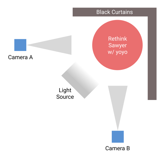
The overall hardware setup consists of two high speed cameras, two black curtains, a lighting source, a Rethink Sawyer robot, and a Duncan Reflex yoyo as shown in Figure below.
AprilTags, a popular choice of visual fiducial tags, are attached on both sides of the yoyo, which are tracked by the two cameras. Although AprilTags are only used for tracking yoyo position and velocity for now, it could potentially be used to capture the yoyo rotation angle in the future.
A fast-moving object usually introduces motion blur with a low-speed camera, which blurs the AprilTags. Therefore, high-speed cameras are needed for keeping track of the AprilTags. Camera A is the EO-0513 USB 3.0 camera from Edmund Optics with a maximum frame rate of 571 FPS. Due to the recent shortage of chips, we were not able to order the second camera with the same model, so instead, we purchased a camera from a different brand with similar specifications. Camera B is the Blackfly S USB3 camera with a maximum frame rate of 522 FPS. Two black curtains are placed behind the robot to reduce background noise when detecting AprilTags. A light source is also used to provide a better and more stable lighting condition for detecting AprilTags.
Different approaches have been tested for tracking yoyo, including (1) Tracking by yoyo color. (2) Tracking by background subtraction (3) Tracking using AprilTags. The yoyo is free to rotate along the string when playing. The shape facing the cameras can change during the rotation, making it hard to find a stable center for color or shape tracking. However, AprilTag also has its own pitfall when used for tracking. It can only be seen when facing the camera within 45 degrees. Therefore, one solution is to attach AprilTags on both sides of the yoyo and place two cameras perpendicular to each other, as shown in Figure 2. This approach ensures that there is always at least one tag being seen by one camera during yoyo playing. The two cameras are running in parallel with a centralized tracking node taking measurements from both cameras. The camera that outputs meaningful measurement is used for the yoyo measured position in the current timestamp.
There are various types of AprilTag families with the trade-off between false-positive rates and tracking distance. The AprilTag family used in this system is “tag25h9”, which contains less bit information for longer distance detection than other families. Since there is no other AprilTag presented in the view, there is no need to worry about the false-positive issue.
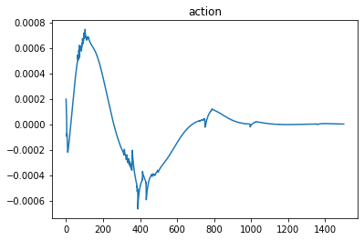
One end of the yoyo string is attached to the end effector of the Rethink Sawyer. The Rethink Saywer end-effector can move up and down to apply control to the yoyo. We need to determine the joint action (could be torque or velocity) to produce the desire end-effector motion calculated by the model in the Simple Yoyo Model section. For the current status, we assume that the yoyo only has vertical movement and ignore the horizontal plane movement. To enforce the assumption, the end-effector movement is constrained in a single vertical line. The end-effector is controlled by velocity, so inverse velocity kinematics is needed to calculate the corresponding joint velocity. The joint velocity vector $\dot{\theta}$ can be calculated by
$\dot{\theta}=M^{-1} J^{\mathrm{T}}\left(J M^{-1} J^{\mathrm{T}}\right)^{-1} \mathcal{V}_{d}$
with $M$ being the weight matrix, $J$ being the Jacobian and ${V}_{d}$ being the desired velocities.
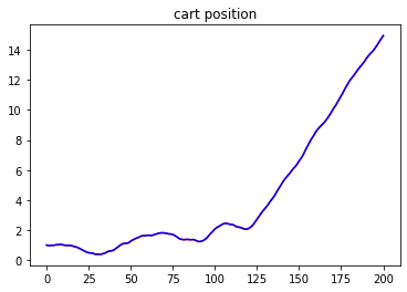
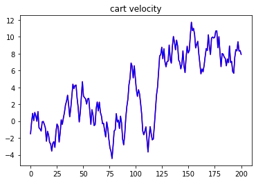
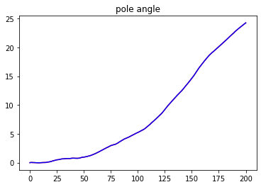
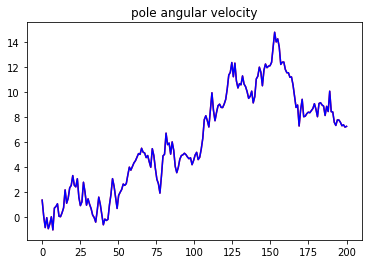
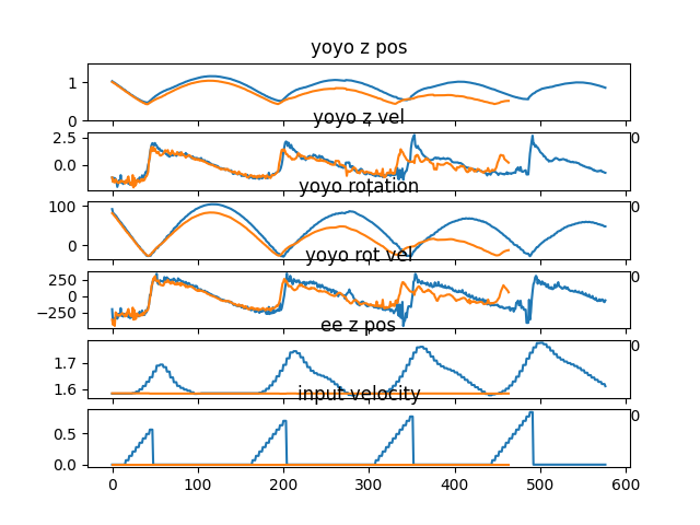
To show that the simple controller can inject energy into the yoyo motion, a comparison was performed with the result shown in Figure 3. The yoyo was released without any control for the orange curve, so it died out in three to four cycles. For the blue curve, the yoyo was controlled by the simple controller. It is obvious that the blue curve shows promising trend for playing yoyo.
Demo Video Again:
This is just a project for validating the yoyo playing task on Sawyer. It shows that the pipeline is working and ready to merge with the upcoming research project which will be posted later.
[1] Jin, Hui-Liang, and Miriam Zacksenhouse. “Robotic yoyo playing with visual feedback.” IEEE transactions on robotics 20.4 (2004): 736-744.
[2] Jin, Hui-Liang, and Miriam Zackenhouse. “Yoyo dynamics: Sequence of collisions captured by a restitution effect.” J. Dyn. Sys., Meas., Control 124.3 (2002): 390-397.
]]>In some scenarios, it is more useful to perform control to cover an area of the state space rather than reach a single point. For example, we might want to command a robot to explore a specific area during a space mission. It could also be useful for reinforcement learning “exploration vs. exploitation” problem, which could aid the policy search process to help faster converging. Additionally, one can also specify a forbidden area so that robot can avoid it during exploration. Model predictive control (MPC) with Kullback–Leibler (KL) ergodic measure can help achieve these goals.
In this project, I implemented the KL ergodic MPC in C++ to achieve real time (100Hz) distribution matching. Three examples are provided to show the ability of this algorithm.
Specifically, sample-based KL-divergence measure is used with ergodic control as described in [1]. In ergodic control, time spent during the trajectory of the robot is proportional to the measure of information gain in that region. Therefore, one can specify a region for a dynamical system to cover. KL-divergence allows us to use ergodic measure in high-dimensional tasks.
This project is just one part of a larger research project Teaching a robot to play yoyo from demonstrations.
The goal of the MPC is to optimize the KL-Ergodic objective with respect to the target area distribution $p$.
Taking notation from [1], given a search domain $\mathcal{S}^{v} \subset \mathbb{R}^{n+m}$, approximated time-averaged current statistics of the robot state is defined by
$q(s \mid x(t))=\frac{1}{t_{f}-t_{0}} \int_{t_{0}}^{t_{f}} \frac{1}{\eta} \exp \left[-\frac{1}{2}|s-\bar{x}(t)|_{\Sigma^{-1}}^{2}\right] d t$
where $\Sigma \in \mathbb{R}^{v \times v}$ is a positive definite matrix that describes the width of the Gaussian. $\eta$ is a normalization constant.
The KL-divergence with ergodic objective is defined by
$D_{\mathrm{KL}}(p | q) =\int_{\mathcal{S}^{v}} p(s) \log \frac{p(s)}{q(s)} d s$
$=\int_{\mathcal{S}^{v}} p(s) \log p(s) d s-\int_{\mathcal{S}^{v}} p(s) \log q(s) d s$
$=-\int_{\mathcal{S}^{v}} p(s) \log q(s) d s$
$\approx-\sum_{i=1}^{N} p\left(s_{i}\right) \log q\left(s_{i}\right)$
$\propto-\sum_{i=1}^{N} p\left(s_{i}\right) \log \int_{t_{0}}^{t_{f}} \exp \left[-\frac{1}{2}\left|s_{i}-\bar{x}(t)\right|_{\Sigma^{-1}}^{2}\right] d t$
In demo 1, I tried to control a point mass in a continuous environment to explore two Gaussian distributions. The states are the current x and y position as well as x and y velocity. The control is the acceleration in the x and y direction. Note that it is possible to define any arbitrary distribution other than Gaussian. In a 2D continuous space spans from -5 to 5 in both x axis and y axis, I defined two Gaussian distributions with mean at (-3,-3) and (2,-1) as well as the variances being (0.5,0.5) and (0.8,0.8), respectively. One distribution is wider than the other one, so we should expect that the agent will explore the wider area with more freedom. The following plot shows a visualization of the distribution.
The agent will start from the origin (0,0) and explore the target distribution. The trajectory is shown in red.
In demo 2, I still tried to control a point mass in a continuous environment. However, this time, there is a moving distribution. It could be a human or a vehicle, which we would like to avoid during our exploration. All other areas will be defined as density 1.0, while there will be a flipped Gaussian with the mean at the center of the moving object. Our goal is to cover the space as much as we can but avoid the moving object during the process. As the gif shows, the agent is actively exploring the state space while avoiding the moving distribution.
In demo 3, I applied the KLE-MPC to the cartpole system, which is a more challenging system than the point mass to demonstrate the ability of this approach.
The states of the cartpole system are: cart x position, cart x velocity, pole theta position, pole theta velocity. The following plot shows a distribution that I would like the cartpole to cover. It is a Gaussian distribution with a mean at x=-0.5, theta=0.0 and variances being 0.1 at x and 0.008 at theta. We would like to only have a small exploration range in the theta state. The following plot shows a visualization of the distribution.
The initial position of the cartpole is at x=-0.5, theta=0.0. It should moving from the position and moving around the target distribution. The following plot shows a visualization of the trajectory of the cartpole trying to cover the distribution. Although it is a little bit too aggressive, which exceeds the distribution but in the acceptable range.
The following is the plot for each state and action. The x state is oscillating around x=-0.5 which matches the mean of the distribution.
This project is just a small scope of a larger research project. The project is still under development, so the source code will be released later. Before that, if you are interested, please feel free to contact me.
[1] Abraham, Ian, Ahalya Prabhakar, and Todd D. Murphey. “An ergodic measure for active learning from equilibrium.” IEEE Transactions on Automation Science and Engineering (2021).
]]>Simultaneous localization and mapping (SLAM) in robotics is the problem of building a map of an unknown environment while estimating an agent’s location at the same time. It has been a hot topic for many years in robotics research. It is a difficult chicken-or-egg problem. Typically, you will need a map for knowing where you are, and you will need a pose to map an environment. SLAM performs the two parts at the same time. SLAM is especially useful in environment where there is no access to GPS or need for higher percision than GPS (indoor, ourdoor, underwater, etc).
Many different SLAM approaches has been developed throughout the years. This project focuses on using Extended Kalman Filtered (EKF) SLAM as the core component with unsupervised learning for extracting landmarks and associating unknown landmarks data. It is worth mentioning that the project is built from scratch using ROS with C++. The only libraries being used are standard C++ library and Armadillo linear algebra library.
Here is a demo video. For more technical details, please scroll down.
The overall pipeline of the project is:
The steps can be summarized as the following:
The project consists of six ROS packages:
nurtle_description
:Adapts the URDF model of turtlebot3 to display it in rvizrigid2d
: A library for performing 2D rigid body transformationstrect
: A feedback controller for following waypointsnuturtle_robot
: Provides interface and interaction with turtlebot hardwarenurtlesim
: Creates kinematic simulation for a diff drive turtlebotnuslam
: Runs the EKF SLAMAll the notes are adapted from [1]
The state of the robot at time t is
$$q_t = \begin{bmatrix} \theta_t \\\ x_t \\\ y_t \end{bmatrix}$$
The state of the map (landmarks) at time t is
$$m_t = \begin{bmatrix} m_x1 \\\ m_y1 \\\ m_x2 \\\ m_y2 \\\ … \\\ m_xn \\\ m_yn \end{bmatrix} \in R^{2n}$$
The combined state is
$$\zeta_t = \begin{bmatrix} q_t \\\ m_t \end{bmatrix} \in R^{2n+3}$$
The input will be current state and current covariance.
$$ \zeta_{t-1}, \Sigma_{t-1} $$
The output will be next state and next covariance
$$ \zeta_{t}, \Sigma_{t} $$
The EKF-SLAM consists of two steps: prediction and correction.
In prediction steps, the estimation comes from the motion commands and odometry updates. Let u_t be the commanded twist computed from encoder readings, update the estimation using the model
$$\zeta_{t}^{-} = g(\zeta_{t-1}, u_t, 0)$$
Propagate the uncertainty:
$$ \Sigma_{t}^{-} = A_t\Sigma_{t-1}A_{t}^{T} + Q $$
where Q is the process noise for the robot motion model
Compute the theoretical measurement (landmark locations) using the current state estimation from correction $$ \hat{z_{t}^{i}} = h_j(\zeta_{t}^{-}) $$
Compute the Kalman gain
$$K_i = \Sigma_{t}^{-}H_{i}^{T}(H_{i}\Sigma_{t}^{-}H_{i}^{T} + R)^{-1}$$
where R is the sensor noise
Compute the posterior state estimation update based on the measurment
$$\zeta_{t} = \zeta_{t}^{-} + K_{i}(z_{t}^{i} - \hat{z_{t}^{i}})$$
Compute the posterior covariance
$$ \Sigma_{t} = (I - K_{i}H_{i})\Sigma_{t}^{-} $$
After receving laser-scan points distance, there will be three problems:
The landmark detection step is designed to solve these three problems.
The laser-scan points will be clustered into groups based on their similarities. A threshold of difference is set between points. If the distance differences between points are small, the points are in the same group.
A circle regression (circle fitting) algorithm from [2] is implemented. When a group of laser-scan points detects a landmark, they will usually be an arc of the circle. The goal of this algorithm is to fit this arc of the circle into a circle function so that the center of the circle can be located.
A classification algorithm from [3] is implemented. This algorithm determines if a cluster of points comes from a circle or not. Let P1 and P2 be the endpoints of a cluster. Let P be any point in the cluster. If the cluster comes from a circle, the angle of PP1P2 is always the same for all P (Inscribed angle theomrem)
After determining the location of the clusters of laser-scan measurement from landmark detection, it is important to associate the measurements with proper features in the map. Due to noise and uncertanties, the measurement for the same landmark will be different every time. Therefore, it is difficult and necessary to confirm which measurement belongs to which landmark. The core idea of unknown data association in this project is to use Mahalanobis distance.
The Mahalanobis distance can be calculated as the following:
$$D = (x_a - x_b)^{T}\Sigma^{-1}(x_a - x_b)$$
It is used to find the distance between measurement from current state and new measurement. The basic idea is: If the new measurement is closed to one of the current landmark state, then the measurement belongs to this landmark. If the new measurement is far away from any landmarks that are currently known, then it will be a new landmark. The threshold will need to be tuned.
In the experiment, the robot drives along closed path in a tube_world with several landmarks with the following environment parameters:
Visualization Elements:
The SLAM path is always following the actual path while the odom is off, proving that SLAM is working.
Position Comparison
Path Type | x (m) | y(m) | z(m) |
---|---|---|---|
Actual | 0.0402 | 0.00288 | 0.0 |
Odom | 0.04953 | -0.0437 | 0.0 |
Slam | 0.04135 | 0.003605 | 0.0 |
Error Percentage Comparing with Actual
Path Type | x (%) | y (%) | z (%) |
---|---|---|---|
Actual | 0.0 | 0.0 | 0.0 |
Odom | 23.2 | 1517.6 | 0.0 |
Slam | 2.86 | 25.2 | 0.0 |
Visualization Elements:
The SLAM estimate is way better than the odomometry.
Position Comparison
Path Type | x (m) | y(m) | theta (rad) |
---|---|---|---|
Actual | 0.0 | 0.0 | 0.0 |
Odom | -0.2845 | -0.38196 | 2.3296567 |
Slam | 0.2687 | -0.19816 | -0.9327513 |
The source code for this implementation can be found here
[1] Notes of Northwestern University ME495 Sensing, Navigation, and Machine Learning for Robotics by Professor Matthew Elwin
[2] A. Al-Sharadqah and N. Chernov, Error Analysis for Circle Fitting Algorithms, Electronic Journal of Statistics (2009), Volume 3 p 886-911
[3] J. Xavier et. al., Fast line, arc/circle and leg detection from laser scan data in a Player driver, ICRA 2005
This project demonstrates the algorithm for learning a system model with a data-drive approach called the Koopman operator and controlling it in a receding horizon manner. This approach learns the system model in a highly efficient way. For example, it is able to capture the system model and apply correct control to keep the cartpole upright with only 300 timesteps in a continuous environment. By using the same pipeline, it can be generalized to other dynamical systems as well.
I implemented the receding horizon controller in with conjugate gradient descent as well as the Koopman operator from scratch. The code has both Python version for demo purposes and C++ version for real-time control purposes. I keep the library usage to minimal so that it is more straight forward to understand. A demo is shown in a continuous cartpole environment.
The Koopman operator is an infinite dimensional linear operator that can describe the propagation of a nonlinear system [1]. Consider a discrete-time dynamical system with nonlinear transformation:
$x_{t+1} = f(x_{t})$
where $x_{k} \in S$ is the state of the system, and $f$ is the transformation $S \rightarrow S$ that propagates the state.
The Koopman operator $K \in C^{NxN}$ can be defined as:
$Kg=g \circ \mathbf{f}$
where $g\in \mathbb{G}: S \rightarrow C$ is the observable of the system.
The Koopman operator has infinite dimensions. It can be approximated using linear finite dimensional operator. The method used to calculate the Koopman operator is the Extended Dynamic Mode Decomposition (EDMD) [2]
Using the Koopman operator for predicting dynamics model is defined as
$\Psi(x_{k+1}) \approx \hat{K}^{\mathrm{T}} \Psi\left(x_{k}\right)^{\mathrm{T}}$
where $\Psi(x)=g(x)$ is a vector of the basis functions defined by the user.
Based on the Koopman operator obtained, for demo purpose, we will formulate and solve an optimal control problem with a quadratic cost. However, other cost or constraint can also be used depends on the problem type.
$f\left(x_{t}, u_{t}\right)=x_{t}^{\top} Q x_{t}+u_{t}^{\top} R u_{t}$
with Q being positive semidefinite and R being positive definite for design tuning
When solving the optimal control, the optimization problem is solved in a conjugate gradient descent manner, which usually converges faster than the steepest descent method.
This article provides a good introduction to conjugate gradient descent https://towardsdatascience.com/complete-step-by-step-conjugate-gradient-algorithm-from-scratch-202c07fb52a8
The demo gym environment is a cartpole system with continuous states and continuous actions.
In the training phase, I first let the agent explore the system with random actions for 3 episodes and 100 time step for each episode.
Then, I tested the environment for 200 timesteps with random actions to see if the model could predict the behavior of the cartpole system.
In the plot, the blue curves are the predictions and the red curves are the ground truths. They are identical. Therefore, we can conclude that the Koopman operator has successfully captured the model.
We are now ready to apply control with the model. The prediciton horizon will be 50 steps, and the demo will run for total 1500 steps. The goal is to move the cartpole from cartpole position x=-1 to the origin x=0 while keeping the pole position upright.
Here are the result state plots
And the control action plot
From the plots, we can conclude that the pipeline successfully learns the cartpole system model and applies correct control that moves the system to the desired final state.
It is worth mentioning that the python version is relatively slow. If real-time control is needed, I will recommended using the C++ version which can run the cartpole system at about 100Hz.
[1]Mauroy, Alexandre, Igor Mezić, and Yoshihiko Susuki, eds. The Koopman Operator in Systems and Control: Concepts, Methodologies, and Applications. Vol. 484. Springer Nature, 2020.
[2]Williams, Matthew O., Ioannis G. Kevrekidis, and Clarence W. Rowley. “A data–driven approximation of the koopman operator: Extending dynamic mode decomposition.” Journal of Nonlinear Science 25.6 (2015): 1307-1346.
]]>