
Data-driven Receding Horizon Control with the Koopman Operator
Project Description
This project demonstrates the algorithm for learning a system model with a data-drive approach called the Koopman operator and controlling it in a receding horizon manner. This approach learns the system model in a highly efficient way. For example, it is able to capture the system model and apply correct control to keep the cartpole upright with only 300 timesteps in a continuous environment. By using the same pipeline, it can be generalized to other dynamical systems as well.
I implemented the receding horizon controller in with conjugate gradient descent as well as the Koopman operator from scratch. The code has both Python version for demo purposes and C++ version for real-time control purposes. I keep the library usage to minimal so that it is more straight forward to understand. A demo is shown in a continuous cartpole environment.
The Koopman Operator
The Koopman operator is an infinite dimensional linear operator that can describe the propagation of a nonlinear system [1]. Consider a discrete-time dynamical system with nonlinear transformation:
$x_{t+1} = f(x_{t})$
where $x_{k} \in S$ is the state of the system, and $f$ is the transformation $S \rightarrow S$ that propagates the state.
The Koopman operator $K \in C^{NxN}$ can be defined as:
$Kg=g \circ \mathbf{f}$
where $g\in \mathbb{G}: S \rightarrow C$ is the observable of the system.
The Koopman operator has infinite dimensions. It can be approximated using linear finite dimensional operator. The method used to calculate the Koopman operator is the Extended Dynamic Mode Decomposition (EDMD) [2]
Using the Koopman operator for predicting dynamics model is defined as
$\Psi(x_{k+1}) \approx \hat{K}^{\mathrm{T}} \Psi\left(x_{k}\right)^{\mathrm{T}}$
where $\Psi(x)=g(x)$ is a vector of the basis functions defined by the user.
Receding Horizon Control with Conjugate Gradient Descent
Based on the Koopman operator obtained, for demo purpose, we will formulate and solve an optimal control problem with a quadratic cost. However, other cost or constraint can also be used depends on the problem type.
$f\left(x_{t}, u_{t}\right)=x_{t}^{\top} Q x_{t}+u_{t}^{\top} R u_{t}$
with Q being positive semidefinite and R being positive definite for design tuning
When solving the optimal control, the optimization problem is solved in a conjugate gradient descent manner, which usually converges faster than the steepest descent method.
This article provides a good introduction to conjugate gradient descent https://towardsdatascience.com/complete-step-by-step-conjugate-gradient-algorithm-from-scratch-202c07fb52a8
Demo
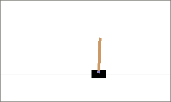
The demo gym environment is a cartpole system with continuous states and continuous actions.
In the training phase, I first let the agent explore the system with random actions for 3 episodes and 100 time step for each episode.
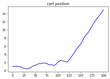
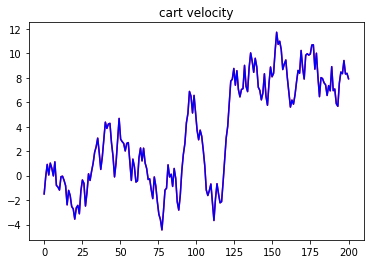
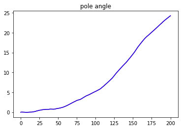
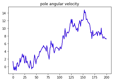
Then, I tested the environment for 200 timesteps with random actions to see if the model could predict the behavior of the cartpole system.
In the plot, the blue curves are the predictions and the red curves are the ground truths. They are identical. Therefore, we can conclude that the Koopman operator has successfully captured the model.
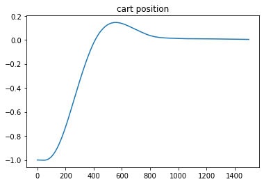
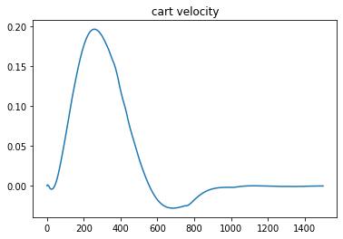
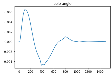
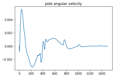
We are now ready to apply control with the model. The prediciton horizon will be 50 steps, and the demo will run for total 1500 steps. The goal is to move the cartpole from cartpole position x=-1 to the origin x=0 while keeping the pole position upright.
Here are the result state plots
And the control action plot
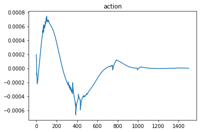
From the plots, we can conclude that the pipeline successfully learns the cartpole system model and applies correct control that moves the system to the desired final state.
Source Code
It is worth mentioning that the python version is relatively slow. If real-time control is needed, I will recommended using the C++ version which can run the cartpole system at about 100Hz.
Reference
[1]Mauroy, Alexandre, Igor Mezić, and Yoshihiko Susuki, eds. The Koopman Operator in Systems and Control: Concepts, Methodologies, and Applications. Vol. 484. Springer Nature, 2020.
[2]Williams, Matthew O., Ioannis G. Kevrekidis, and Clarence W. Rowley. “A data–driven approximation of the koopman operator: Extending dynamic mode decomposition.” Journal of Nonlinear Science 25.6 (2015): 1307-1346.