EKF-SLAM with Machine Learning

Project Description

Simultaneous localization and mapping (SLAM) in robotics is the problem of building a map of an unknown environment while estimating an agent’s location at the same time. It has been a hot topic for many years in robotics research. It is a difficult chicken-or-egg problem. Typically, you will need a map for knowing where you are, and you will need a pose to map an environment. SLAM performs the two parts at the same time. SLAM is especially useful in environment where there is no access to GPS or need for higher percision than GPS (indoor, ourdoor, underwater, etc).

Many different SLAM approaches has been developed throughout the years. This project focuses on using Extended Kalman Filtered (EKF) SLAM as the core component with unsupervised learning for extracting landmarks and associating unknown landmarks data. It is worth mentioning that the project is built from scratch using ROS with C++. The only libraries being used are standard C++ library and Armadillo linear algebra library.

Here is a demo video. For more technical details, please scroll down.

Overview

Pipeline

The overall pipeline of the project is:

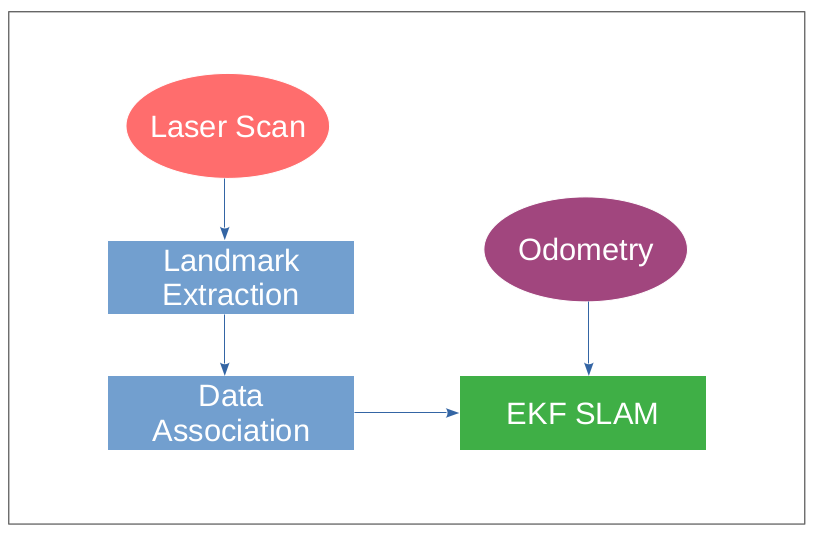
The steps can be summarized as the following:

1. The turtlebot laser scan first need to be programmed to detect landmarks and wall shapes
2. Each data point will be grouped into different landmarks or walls using clustering
3. Using the algorithm in [2] to perform circle regression to extract the landmarks location based on each cluster of laser scan points
4. Using the algorithm in [3] to classify the clusters of points into wall or cylinder landmark
5. Associating data to landmarks using mahalanobis distance
6. Perform odometry calculation
7. Update EKF-SLAM using associated landmark position and odometry information

Modules

The project consists of six ROS packages:

1. nurtle_description:Adapts the URDF model of turtlebot3 to display it in rviz
2. rigid2d: A library for performing 2D rigid body transformations
3. trect: A feedback controller for following waypoints
4. nuturtle_robot: Provides interface and interaction with turtlebot hardware
5. nurtlesim: Creates kinematic simulation for a diff drive turtlebot
6. nuslam: Runs the EKF SLAM

Technical Highlights

All the notes are adapted from [1]

EKF-SLAM

The state of the robot at time t is

$$q_t = \begin{bmatrix} \theta_t \\\ x_t \\\ y_t \end{bmatrix}$$

The state of the map (landmarks) at time t is

$$m_t = \begin{bmatrix} m_x1 \\\ m_y1 \\\ m_x2 \\\ m_y2 \\\ … \\\ m_xn \\\ m_yn \end{bmatrix} \in R^{2n}$$

The combined state is

$$\zeta_t = \begin{bmatrix} q_t \\\ m_t \end{bmatrix} \in R^{2n+3}$$

The input will be current state and current covariance.

$$ \zeta_{t-1}, \Sigma_{t-1} $$

The output will be next state and next covariance

$$ \zeta_{t}, \Sigma_{t} $$

The EKF-SLAM consists of two steps: prediction and correction.

Prediction

In prediction steps, the estimation comes from the motion commands and odometry updates. Let u_t be the commanded twist computed from encoder readings, update the estimation using the model

$$\zeta_{t}^{-} = g(\zeta_{t-1}, u_t, 0)$$

Propagate the uncertainty:

$$ \Sigma_{t}^{-} = A_t\Sigma_{t-1}A_{t}^{T} + Q $$

where Q is the process noise for the robot motion model

Correction for each Measurment i

Compute the theoretical measurement (landmark locations) using the current state estimation from correction $$ \hat{z_{t}^{i}} = h_j(\zeta_{t}^{-}) $$

Compute the Kalman gain

$$K_i = \Sigma_{t}^{-}H_{i}^{T}(H_{i}\Sigma_{t}^{-}H_{i}^{T} + R)^{-1}$$

where R is the sensor noise

Compute the posterior state estimation update based on the measurment

$$\zeta_{t} = \zeta_{t}^{-} + K_{i}(z_{t}^{i} - \hat{z_{t}^{i}})$$

Compute the posterior covariance

$$ \Sigma_{t} = (I - K_{i}H_{i})\Sigma_{t}^{-} $$

Landmark Detection

After receving laser-scan points distance, there will be three problems:

1. How do we distinguish groups of laser-scan points from different objects
2. What is the location of the landmark that this group of laser scan corresponds to?
3. Are the laser-scan points reflecting from a wall or a landmark?

The landmark detection step is designed to solve these three problems.

1. The laser-scan points will be clustered into groups based on their similarities. A threshold of difference is set between points. If the distance differences between points are small, the points are in the same group.

2. A circle regression (circle fitting) algorithm from [2] is implemented. When a group of laser-scan points detects a landmark, they will usually be an arc of the circle. The goal of this algorithm is to fit this arc of the circle into a circle function so that the center of the circle can be located.

3. A classification algorithm from [3] is implemented. This algorithm determines if a cluster of points comes from a circle or not. Let P1 and P2 be the endpoints of a cluster. Let P be any point in the cluster. If the cluster comes from a circle, the angle of PP1P2 is always the same for all P (Inscribed angle theomrem)

Unknow Data Association

After determining the location of the clusters of laser-scan measurement from landmark detection, it is important to associate the measurements with proper features in the map. Due to noise and uncertanties, the measurement for the same landmark will be different every time. Therefore, it is difficult and necessary to confirm which measurement belongs to which landmark. The core idea of unknown data association in this project is to use Mahalanobis distance.

The Mahalanobis distance can be calculated as the following:

$$D = (x_a - x_b)^{T}\Sigma^{-1}(x_a - x_b)$$

It is used to find the distance between measurement from current state and new measurement. The basic idea is: If the new measurement is closed to one of the current landmark state, then the measurement belongs to this landmark. If the new measurement is far away from any landmarks that are currently known, then it will be a new landmark. The threshold will need to be tuned.

---

Simulation Experiment Result

In the experiment, the robot drives along closed path in a tube_world with several landmarks with the following environment parameters:

• Robot translational commanded twist noise: ~N(0, 0.01)
• Robot rotational commanded twist noise: ~N(0, 0.01)
• Robot wheel minimum slip noise: 0.9
• Robot wheel maximum slip noise: 1.1
• Laser scan range noise: ~N(0,0.005)

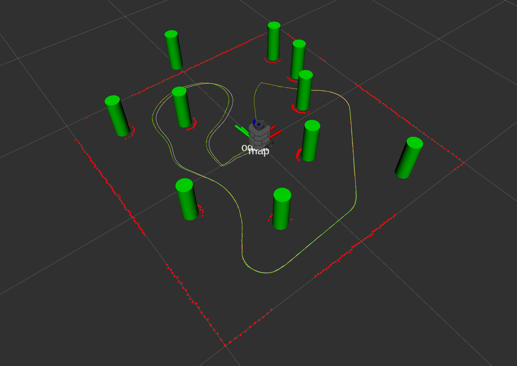
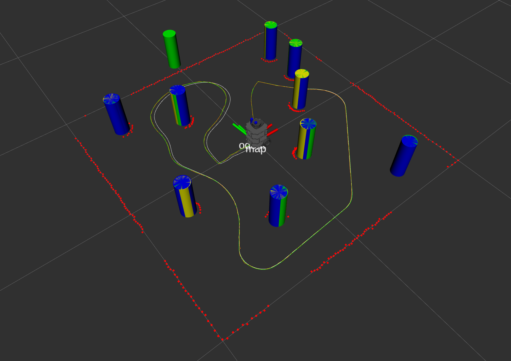
Visualization Elements:

• Green tubes: Ground truth tube positions
• Blue tubes: Current SLAM map
• Yellow tubes: Measurement extracted from laser scan
• Green path: Ground truth path
• White path: Odometry path
• Orange path: SLAM path

Ground Truth Map

SLAM Map

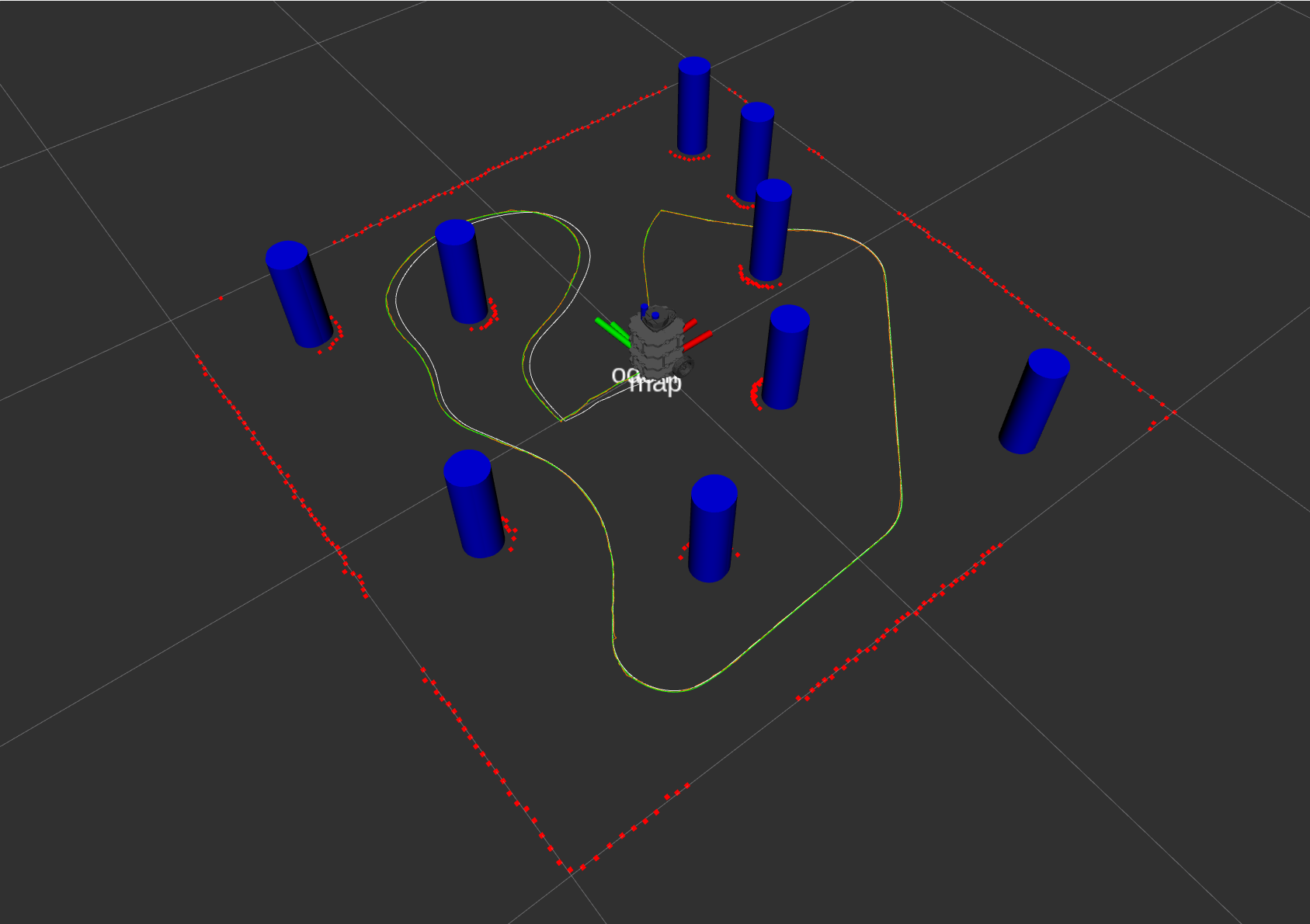
Compare SLAM Map(Blue), Groud Truth(Green), Measurement(Yellow)

Result Analysis

The SLAM path is always following the actual path while the odom is off, proving that SLAM is working.

Position Comparison

Path Type	x (m)	y(m)	z(m)
Actual	0.0402	0.00288	0.0
Odom	0.04953	-0.0437	0.0
Slam	0.04135	0.003605	0.0

Error Percentage Comparing with Actual

Path Type	x (%)	y (%)	z (%)
Actual	0.0	0.0	0.0
Odom	23.2	1517.6	0.0
Slam	2.86	25.2	0.0

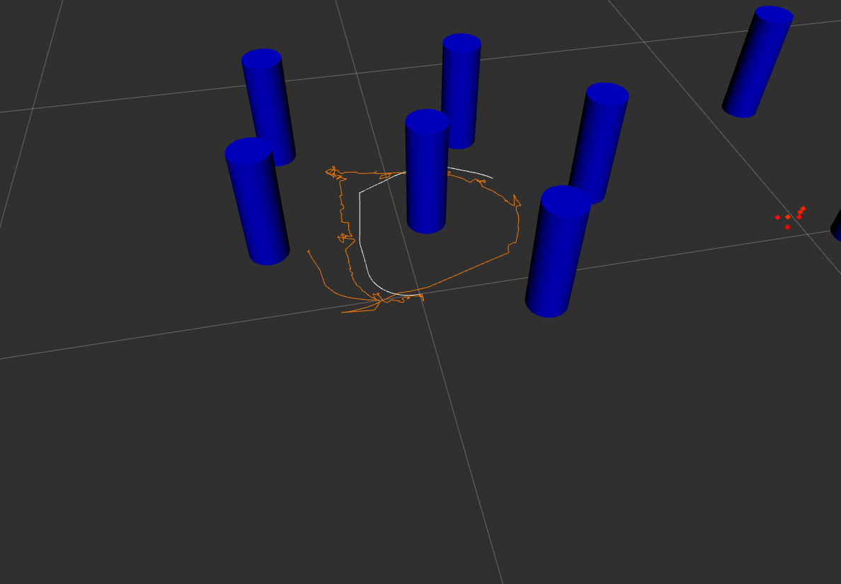
Actual Turtlebot Experiment Result

Visualization Elements:

• Blue tubes: Current SLAM map
• White path: Odometry path
• Orange path: SLAM path

The SLAM estimate is way better than the odomometry.

Result Analysis

Position Comparison

Path Type	x (m)	y(m)	theta (rad)
Actual	0.0	0.0	0.0
Odom	-0.2845	-0.38196	2.3296567
Slam	0.2687	-0.19816	-0.9327513

Source Code

The source code for this implementation can be found here

---

Future Development

1. Wheel odometry can be replaced with a visual odometry
2. Drop the assumption of cylindrical landmarks and use occupation grid

---

Reference

[1] Notes of Northwestern University ME495 Sensing, Navigation, and Machine Learning for Robotics by Professor Matthew Elwin
[2] A. Al-Sharadqah and N. Chernov, Error Analysis for Circle Fitting Algorithms, Electronic Journal of Statistics (2009), Volume 3 p 886-911
[3] J. Xavier et. al., Fast line, arc/circle and leg detection from laser scan data in a Player driver, ICRA 2005