
Planning & Prediction with Human Preference via Deep Inverse Reinforcement Learning
Project Description
Many Reinforcement Learning (RL) algorithms assume that a reward function is known (or can be obtained by interacting with the environment). However, it is hard to define such a reward function that leads to desired behaviors in many cases. It could be due to sparse reward, high dimensionality, etc. There is a gap between human understanding of reward and the way that RL algorithm finds policy based on the reward. Therefore, it will be beneficial to be able to determine reward function from human demonstration. It is similar to a translator that converts human intent to a robot’s reward function. Moreover, by extracting the reward function from human demonstrations, we will also be able to infer the human preference. For example, a human demonstrator might like moving very close to a wall when approaching the goal. An agent can learn from demonstration to have a higher reward close to the wall but still maintain the appropriate weight ratio with respect to the goal reward, which ends up leading the agent to the goal along the wall. Even when the environment has changed (wall position has changed), the agent can still move with the same preference (closed to the wall), which is the ability to generalize to a novel configuration of the environment. With such a reward function, we can predict human behavior based on preference for similar environments. Another example would be in autonomous driving where the vehicle can learn human driving preference and mimic similar behavior to generate a preferred and comfortable driving trajectory.
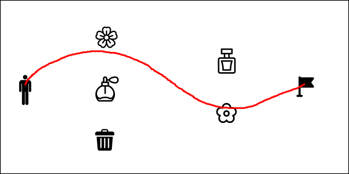
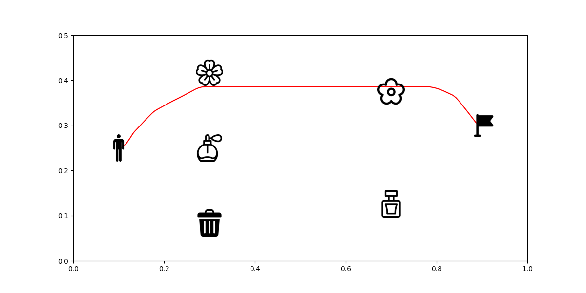
This project uses Maximum Entropy Deep Inverse Reinforcement Learning (IRL) with Soft Actor-Critic (SAC) to determine a reward function representing user preference during a continuous path planning scenario. The scenario came up when I walked by a trash can one time, and I was disgusted by the smell. The next time I walked by the same place, I intentionally avoided the trash can (that’s my preference). Figure 1 shows an example. There is a room that has perfumes, natural flowers, and a trash bag. A person needs to navigate through perfumes, flowers, or trash bags in order to reach his/her goal. These objects have different smells which correspond to different preferences when the person chooses a path: Some people like natural smell from flowers, some people like artificial smell from perfumes, and some people might be ok with trash bag smell as long as they can get to the goal. However, we don’t have this information as a prior; we need to infer the preference based on the person’s behavior.
 |
|---|
| Figure 1. An Example Scenario |
The high-level plan is to take a demonstrated path. We then use IRL to extract a reward function from the demonstration for this 2D continuous space. After that, we can use the reward function with standard RL to predict the human preferred path next time he/she enters the room, even when the positions of the objects have changed.
Maximum Entropy Deep IRL
The IRL algorithm used in this project is a modified version of the paper Maximum Entropy Deep Inverse Reinforcement Learning by Wulfmeier et al. in 2016[1]. I will discuss a short version of the algorithm formulation here. For more detail information, please refer to the paper. The following notations are also taken from the paper[1]
In standard RL, we assume a Markov Decision Process (MDP) that is defined by state $S$, action $A$, transition model $T$, and the reward $r$. The policy $\pi$ that maximizes the expected reward is the optimal policy $\pi^{*}$. In IRL, we are interested in the inverse problem: The policy $\pi$ is given which will be used to determine the reward $r$.
How do we express the reward function? In many of the previous IRL algorithms, the reward function is represented by a linear combination of the features.
$$r = \theta^{T}f$$
where $\theta$ is the weight vector and $f$ is the feature vector. The form of Linear combination will limit the ways of representing reward functions since there could be rewards that cannot be approximated by linear formulation. In order to be more generalized to nonlinear reward functions, we can use neural network as a nonlinear function approximators. This is where the term “Deep” comes up in this algorithm compared to its predecessor Maximum Entropy IRL by Ziebart et al. in 2008[2]. The reward function now becomes:
$$r=g(f, \theta_{1}, \theta_{2}, …)$$
where $\theta_{n}$ are just the network parameters in the neural network.
To solve the IRL problem, we will maximize the joint posterior distribution of the demonstration $D$ and the network parameters given the reward function:
$$ L(\theta)=\log P(D, \theta \mid r) = \log P(D \mid r) + \log P(\theta) = L_{D} + L_{\theta}$$
Since it is differentiable with respect to $\theta$, we can take the gradient with respect to $\theta$ and use gradient descent.
$$ \frac{\partial L}{\partial \theta}=\frac{\partial L_{D}}{\partial \theta}+\frac{\partial L_{\theta}}{\partial \theta} $$
The first term can be further decomposed into:
$$ \frac{\partial L_{D}}{\partial \theta}=\frac{\partial L_{D}}{\partial r} \cdot \frac{\partial r}{\partial \theta} $$
Based on the the original Maximum Entropy IRL [2]:
$$ \frac{\partial L_{D}}{\partial r} = \left(\mu_{D}-\mathbb{E}[\mu]\right) $$
which is the difference between the expert demonstration features trajectories and the expected current policy features trajectories. The difference here can be used as the error that starts the back propagation.
Implementation
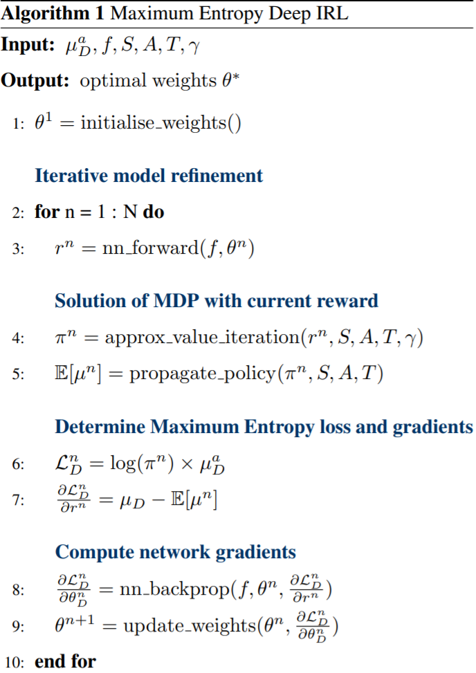
The implementation is based on the algorithm given by the original paper as shown in Figure 2 with modifications.
 |
|---|
| Figure 2. Full Algorithm |
The modifications happen at line 4 and line 5 in Figure 2. Line 4 is used for determining the current optimal policy given the current reward function. Line 5 is for generating expected state features based on the current optimal policy. However, the original paper uses value iteration to find the optimal policy, which is difficult in a continuous environment. To adapt to continuous environment and possibly expand to other future robotics applications, I decided to use Soft Actor-Critic (SAC) as the method to find the optimal policy with the current reward function. The complete pipeline is shown in Figure 3
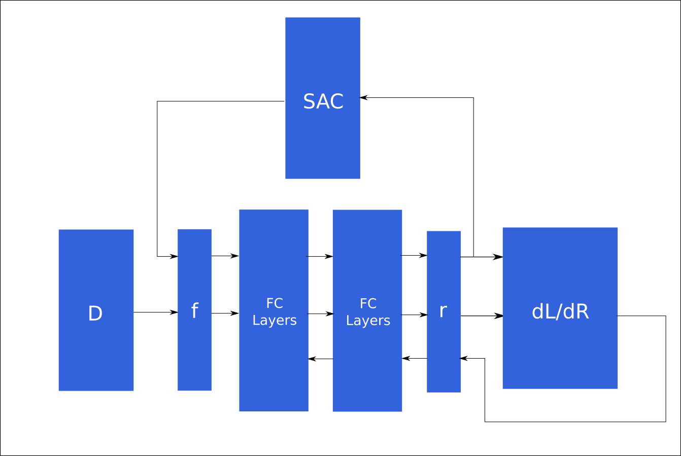 |
|---|
| Figure 3. Full Pipeline for Training |
The pipeline can be described as the following steps:
- Initialize neural network parameters
- Collect user demonstrations
- Obtain feature trajectories from user demonstrations
- Use current reward function from the neural network to obtain current policy
- Obtain current policy feature trajectories
- Take the results from step 3 and step 5, put into the neural network
- Use the output from the neural network to perform back propagation
- Repeat from step 4
The network we will be using is a two-layer network with 64 nodes as the hidden states for each layer.
Experiment
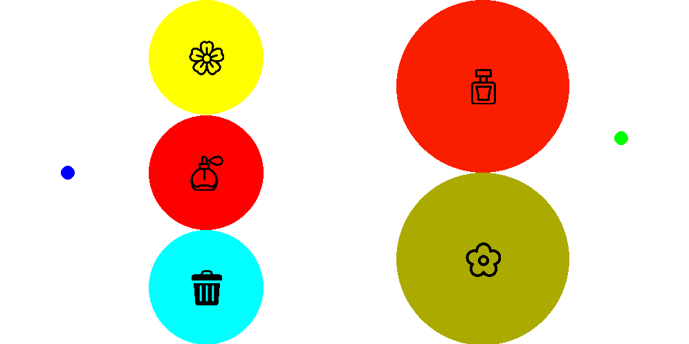
As briefly introduced in the previous section, the scenario will be described in more details here. Figure 4 shows the example scenario again. It is a rectagular 2D continuous space. A human starting from the right side (the blue dot) can take continuous actions to reach the goal (the green dot) on the left side. The human will need to go through two layers of objects including perfumes, flowers, and trash bag. Each of these objects will have different smells which only diffuse to a circular area around the object, and there is no intersection between the smells. The color shows the area each smell covers. The first layer is covered by sakura flowers, perfume 1, and a trash bag (from the top to the bottom). The second layer does not have the trash bag, it is only covered by roses and perfume 2 (from the top to the bottom). A person will navigate to the goal based on his/her preference of smells.
 |
|---|
| Figure 4. An Example Scenario |
To perform the smell room experiment, I first created a game interface for collecting user demonstration using Pygame. A user can use a gaming controller joystick as the input for creating demonstration. Figure 5 shows an example of a user moving freely in the room with a joystick. Once the user thinks the demonstration is complete, the user can close the pygame window, which the trajectory will be recorded.
 |
|---|
| Figure 5. The Pygame Interface |
One example of the demonstration path is shown in Figure 6. We will proceed with this demonstration for the rest of the experiment. From this demonstration, it seems like the user likes the natural smell from flowers. However, we don’t have a correct weighted reward function for this preference. We will use IRL to extract such a reward function.
 |
|---|
| Figure 6. Demonstration Example |
Before doing that, the state trajectory will need to be converted into feature trajectory as the input into the algorithm. There are six features:
- Getting the smell from sakura flower (0 or 1)
- Getting the smell from perfume 1 (0 or 1)
- Getting the smell from trash (0 or 1)
- Getting the smell from rose (0 or 1)
- Getting the smell from perfurm 2 (0 or 1)
- The normalized distance to the goal from the current position
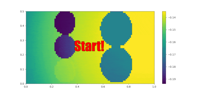
The feature trajectory is then enter the IRL algorithm described in the Implementation section. The number of iteration for the IRL is set to 60. For each IRL iteration, the SAC part will need to run for 30000 iterations to find the current policy. The reward changes during training is recorded as a gif in Figure 7. At the first frame, we can see that the rewards at sakura and perfume 1 are lower than the trash bag. As the training proceeded further, the rewards for sakura started to increase and reached a higher value that the other two smells. At the second layer, the rose smell reward increased rapidly at the beginning, but slowly decreased to a lower value than the goal, which ensured that the agent would not stuck at the second layer and stopped moving forward to the goal.
 |
|---|
| Figure 7. Reward Changes during Training |
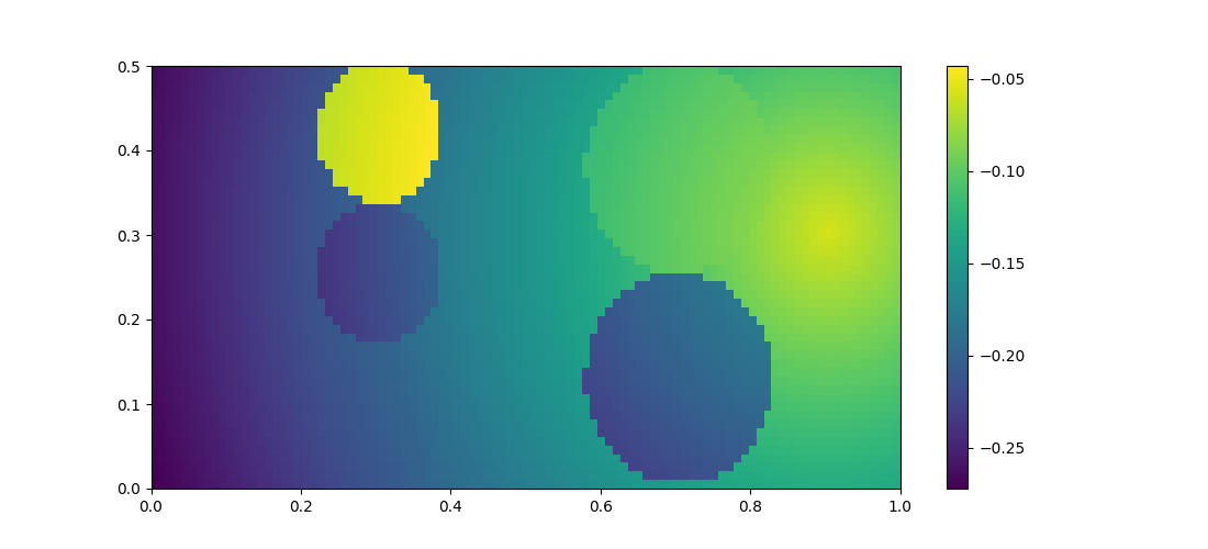
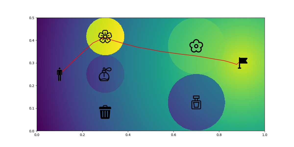
Figure 8 shows the final reward function in the room space. It is obvious to tell that the sakura position has the highest reward at the first layer among all three smells. Unfortunately, for now we won’t be able to distinguish the preference for the other two smells. It would be enough for now to only find the best preference. At the second layer, the roses position has the higher reward than the perfume 2. At the end, the goal position has the highest reward in the space. It shows that the reward function looks promising to be able to successfully encode the preference from the human demonstration path. We will later use this reward to find a policy which can further prove the success.
 |
|---|
| Figure 8. Final Reward |
Figure 9 shows an overlay of the demonstration over the final reward function.
 |
|---|
| Figure 9. Demonstration and Reward |
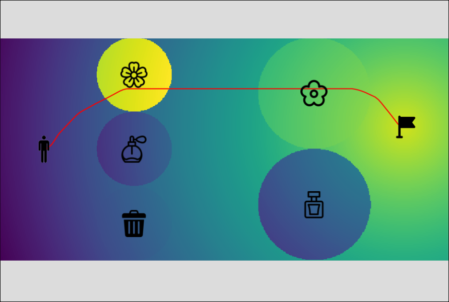
After obtaining the reward function, we will use it to find a policy. If the training is successful, the policy should have the similar preference as the human demonstration. We will run SAC using the reward function for 50000 episodes. Figure 10 shows the result. The predicted path goes through the sakura and rose position which matches the preference from the human demonstrated path. Notice that the predicted path won’t perfectly fit with the demonstrated path since our goal is to match the preference rather than the trajectory.
 |
|---|
| Figure 10. Prediction |
To prove that there is no overfitting, we will show that the algorithm can adapt to changes in the environment configuration. The change happens at the second layer which the positions of the rose and perfume 2 have been switched. We then use SAC to generate a new policy based on the new environment configuration. As expected, the new predicted path still matches the preference even when the environment changes.
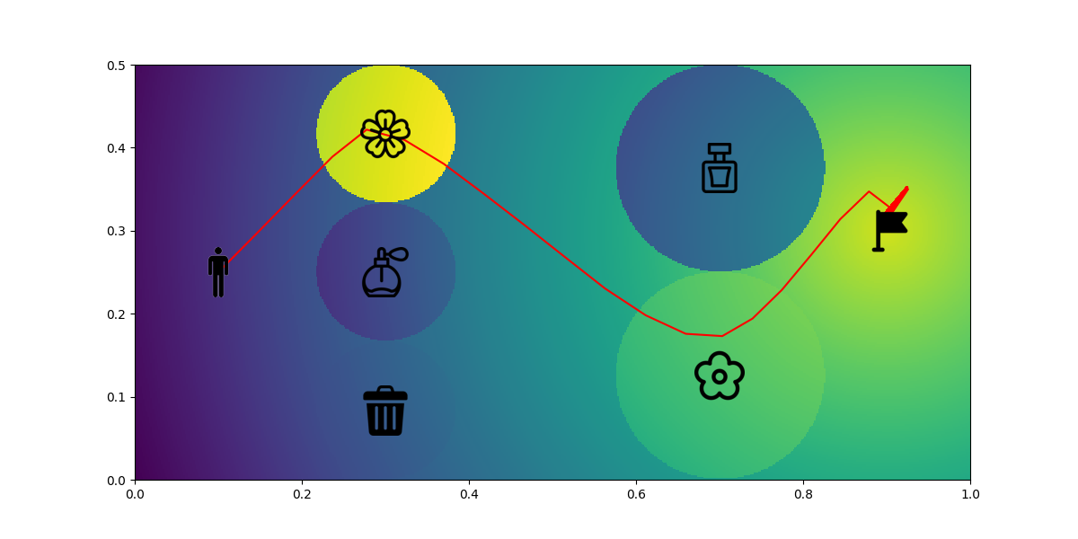 |
|---|
| Figure 11. Environment Change |
We can also change the setup at the first layer to show more examples for generalization. The position switch happen between the sakura and perfume 1. Again as expected, the new predicted path still matches the preference even when the environment changes.
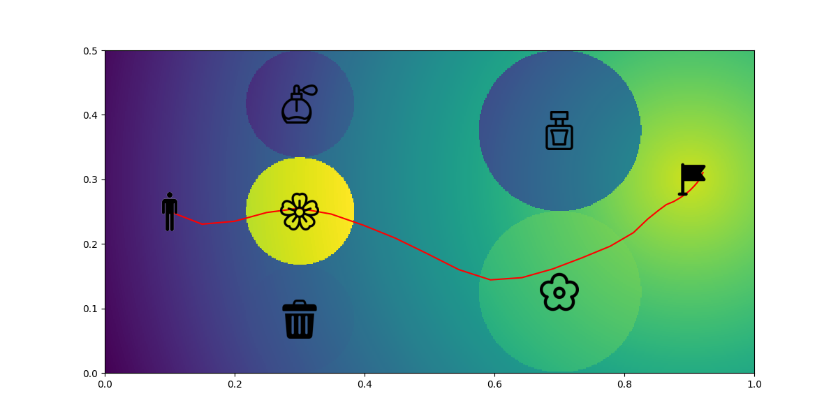 |
|---|
| Figure 12. Environment Change |
Conclusion
This project shows a simple example of using IRL to predict a path based on user preference in a continuous environment. In the future, I would like to make it work on a real robot problem. There are still some pitfalls and room for improvement with this approach.
- It requires more than thousands of training episodes, which will not be realistic on a real robot problem.
- Although there is no need to handcraft the reward function anymore, we need to design the feature for the problem. It is more straightforward for a human engineer to understand and design the feature, but it is still challenging to find the right features for the algorithm to converge.
- Human behavior could be irrational. It would be better to have a parameter that represents the irrationality of the human to account for more unexpected behavior during predictions.
Reference
[1] Wulfmeier, Markus, Peter Ondruska, and Ingmar Posner. “Maximum entropy deep inverse reinforcement learning.” arXiv preprint arXiv:1507.04888 (2015).
[2] Ziebart, Brian D., et al. “Maximum entropy inverse reinforcement learning.” Aaai. Vol. 8. 2008.