
Real-time KL-Ergodic Distribution-based Model Predictive Control
Project Description
In some scenarios, it is more useful to perform control to cover an area of the state space rather than reach a single point. For example, we might want to command a robot to explore a specific area during a space mission. It could also be useful for reinforcement learning “exploration vs. exploitation” problem, which could aid the policy search process to help faster converging. Additionally, one can also specify a forbidden area so that robot can avoid it during exploration. Model predictive control (MPC) with Kullback–Leibler (KL) ergodic measure can help achieve these goals.
In this project, I implemented the KL ergodic MPC in C++ to achieve real time (100Hz) distribution matching. Three examples are provided to show the ability of this algorithm.
- Explore specific targets
- Explore but avoid a moving target
- Cartpole system
Specifically, sample-based KL-divergence measure is used with ergodic control as described in [1]. In ergodic control, time spent during the trajectory of the robot is proportional to the measure of information gain in that region. Therefore, one can specify a region for a dynamical system to cover. KL-divergence allows us to use ergodic measure in high-dimensional tasks.
This project is just one part of a larger research project Teaching a robot to play yoyo from demonstrations.
KL-Ergodic objective
The goal of the MPC is to optimize the KL-Ergodic objective with respect to the target area distribution $p$.
Taking notation from [1], given a search domain $\mathcal{S}^{v} \subset \mathbb{R}^{n+m}$, approximated time-averaged current statistics of the robot state is defined by
$q(s \mid x(t))=\frac{1}{t_{f}-t_{0}} \int_{t_{0}}^{t_{f}} \frac{1}{\eta} \exp \left[-\frac{1}{2}|s-\bar{x}(t)|_{\Sigma^{-1}}^{2}\right] d t$
where $\Sigma \in \mathbb{R}^{v \times v}$ is a positive definite matrix that describes the width of the Gaussian. $\eta$ is a normalization constant.
The KL-divergence with ergodic objective is defined by
$D_{\mathrm{KL}}(p | q) =\int_{\mathcal{S}^{v}} p(s) \log \frac{p(s)}{q(s)} d s$
$=\int_{\mathcal{S}^{v}} p(s) \log p(s) d s-\int_{\mathcal{S}^{v}} p(s) \log q(s) d s$
$=-\int_{\mathcal{S}^{v}} p(s) \log q(s) d s$
$\approx-\sum_{i=1}^{N} p\left(s_{i}\right) \log q\left(s_{i}\right)$
$\propto-\sum_{i=1}^{N} p\left(s_{i}\right) \log \int_{t_{0}}^{t_{f}} \exp \left[-\frac{1}{2}\left|s_{i}-\bar{x}(t)\right|_{\Sigma^{-1}}^{2}\right] d t$
Demo 1 (Explore specific targets)
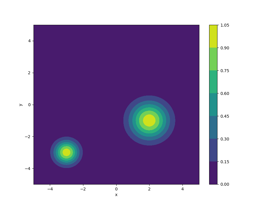
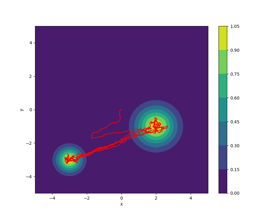
In demo 1, I tried to control a point mass in a continuous environment to explore two Gaussian distributions. The states are the current x and y position as well as x and y velocity. The control is the acceleration in the x and y direction. Note that it is possible to define any arbitrary distribution other than Gaussian. In a 2D continuous space spans from -5 to 5 in both x axis and y axis, I defined two Gaussian distributions with mean at (-3,-3) and (2,-1) as well as the variances being (0.5,0.5) and (0.8,0.8), respectively. One distribution is wider than the other one, so we should expect that the agent will explore the wider area with more freedom. The following plot shows a visualization of the distribution.
The agent will start from the origin (0,0) and explore the target distribution. The trajectory is shown in red.
Demo 2 (Explore but avoid a moving target)
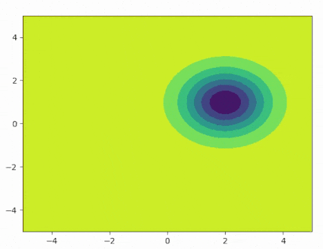
In demo 2, I still tried to control a point mass in a continuous environment. However, this time, there is a moving distribution. It could be a human or a vehicle, which we would like to avoid during our exploration. All other areas will be defined as density 1.0, while there will be a flipped Gaussian with the mean at the center of the moving object. Our goal is to cover the space as much as we can but avoid the moving object during the process. As the gif shows, the agent is actively exploring the state space while avoiding the moving distribution.
Demo 3 (Cartpole)
In demo 3, I applied the KLE-MPC to the cartpole system, which is a more challenging system than the point mass to demonstrate the ability of this approach.
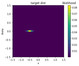
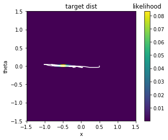
The states of the cartpole system are: cart x position, cart x velocity, pole theta position, pole theta velocity. The following plot shows a distribution that I would like the cartpole to cover. It is a Gaussian distribution with a mean at x=-0.5, theta=0.0 and variances being 0.1 at x and 0.008 at theta. We would like to only have a small exploration range in the theta state. The following plot shows a visualization of the distribution.
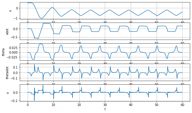
The initial position of the cartpole is at x=-0.5, theta=0.0. It should moving from the position and moving around the target distribution. The following plot shows a visualization of the trajectory of the cartpole trying to cover the distribution. Although it is a little bit too aggressive, which exceeds the distribution but in the acceptable range.
The following is the plot for each state and action. The x state is oscillating around x=-0.5 which matches the mean of the distribution.
Source code
This project is just a small scope of a larger research project. The project is still under development, so the source code will be released later. Before that, if you are interested, please feel free to contact me.
Reference
[1] Abraham, Ian, Ahalya Prabhakar, and Todd D. Murphey. “An ergodic measure for active learning from equilibrium.” IEEE Transactions on Automation Science and Engineering (2021).